Linear response and transmission/reflection coeffictients for magnon three-wave mixing

using HarmonicSteadyState, QuantumCumulants, Plots

Consider a model of nonlinear magnon-magnon coupling, as described in this paper. The model describes a three-wave mixing interaction between a strongly driven $k=0$ FMR mode and two parametricallly excited propagating modes with opposite momentum $\pm k$ and at half frequency. In this notebook, we will show how the mean-field approximation can be used to calculate steady states, and to calculate the $S_{21}$ transmission coefficient.

hm = FockSpace(:magnon)
hc = FockSpace(:polariton)
h = hm ⊗ hc  # Hilbertspace

@qnumbers m::Destroy(h, 1) c::Destroy(h, 2) # Operators

@rnumbers Δ Vk Ωd γm γk # Parameters
param = [Δ, Vk, Ωd, γm, γk]

H_RWA_sym = (
    Δ * m' * m + Δ / 2 * c' * c + Vk * m * c' * c' + Vk * m' * c * c + (Ωd * m + Ωd * m')
)
ops = [m, m', c, c'] # Operators for meanfield evolution

eqs_RWA = meanfield(ops, H_RWA_sym, [m, c]; rates=[γm, γk], order=1)
eqs_completed_RWA = complete(eqs_RWA) # Meanfield equations using QuantumCumulants.jl

\begin{align} \frac{d}{dt} \langle m\rangle &= -1 i \langle c\rangle ^{2} Vk -1 i \Delta \langle m\rangle -1 i {\Omega}d -0.5 {\gamma}m \langle m\rangle \ \frac{d}{dt} \langle m^\dagger\rangle &= 1 i \Delta \langle m^\dagger\rangle -0.5 {\gamma}m \langle m^\dagger\rangle + 1 i {\Omega}d + 1 i Vk \langle c^\dagger\rangle ^{2} \ \frac{d}{dt} \langle c\rangle &= -0.5 \langle c\rangle {\gamma}k + \frac{-1}{2} i \langle c\rangle \Delta -2 i Vk \langle m\rangle \langle c^\dagger\rangle \ \frac{d}{dt} \langle c^\dagger\rangle &= -0.5 {\gamma}k \langle c^\dagger\rangle + \frac{1}{2} i \Delta \langle c^\dagger\rangle + 2 i \langle c\rangle \langle m^\dagger\rangle Vk \end

We can use this meanfield equations to construct a HarmonicEquation object in HarmonicSteadyState.jl. In the construction, additional information is computed, such as the Jacobian of the equations, which is used to determine the stability if the the steady states.

harmonic_eq = HarmonicEquation(eqs_completed_RWA, param)

A set of 4 harmonic equations
Variables: mᵣ(t), mᵢ(t), cᵣ(t), cᵢ(t)
Parameters: Δ, Vk, Ωd, γm, γk

Harmonic ansatz: 
0 = mᵣ(t) + mᵢ(t) + cᵣ(t) + cᵢ(t)

Harmonic equations:

1.4142135623730951(-0.35355339059327373mᵣ(t)*γm - 0.7071067811865475mᵢ(t)*Δ - 0.9999999999999998Vk*cᵣ(t)*cᵢ(t)) ~ Differential(t)(mᵣ(t))

-1.4142135623730951(-Ωd - 0.7071067811865475mᵣ(t)*Δ + 0.35355339059327373mᵢ(t)*γm - 0.4999999999999999Vk*(cᵣ(t)^2) + 0.4999999999999999Vk*(cᵢ(t)^2)) ~ Differential(t)(mᵢ(t))

1.4142135623730951(-0.35355339059327373cᵣ(t)*γk - 0.35355339059327373cᵢ(t)*Δ - 0.9999999999999998Vk*cᵣ(t)*mᵢ(t) + 0.9999999999999998Vk*mᵣ(t)*cᵢ(t)) ~ Differential(t)(cᵣ(t))

-1.4142135623730951(-0.35355339059327373cᵣ(t)*Δ + 0.35355339059327373cᵢ(t)*γk - 0.9999999999999998Vk*cᵣ(t)*mᵣ(t) - 0.9999999999999998Vk*cᵢ(t)*mᵢ(t)) ~ Differential(t)(cᵢ(t))

Let's sweep the power of the drive ${\mathrm{\Omega }}_d$, with $\mathrm{\Delta }=0$, and solve for the steady state. The steady-state solutions show that the FMR mode saturates after a threshold power, followed by the coherent excitation of the parametrically induced counter-propagating modes.

drive_range = range(0, 1.8, 100)
fixed = (Δ => 0, Vk => 0.0002, γm => 0.1, γk => 0.01)
varied = (Ωd => drive_range)
result = get_steady_states(harmonic_eq, TotalDegree(), varied, fixed)

plot(plot(result; y="1/sqrt(2)*(mᵣ+ mᵢ)"), plot(result; y="1/sqrt(2)*(cᵣ + cᵢ)"))

# Linear response and S21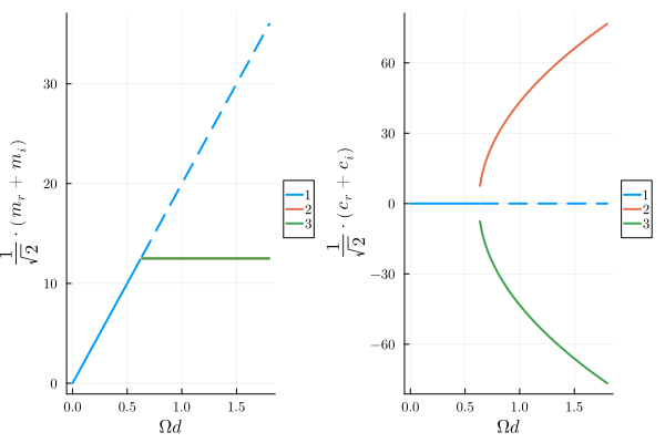

To find the response of the driven system to a second, weak probe, we use the method described here. Here, we calculate the response in the same rotating frame as the Hamiltonian. The linear response is related to the scattering parameter $S_{21}$ by $S_{21}(\omega )=1-\sqrt{{\kappa }_{ext}}\chi (\omega ),$ where ${\kappa }_{ext}$ is the coupling of the system to the measurement apparatus.

The result below shows the characteristic splitting of the magnon resonance above the power threshold, which matches the experiment.

Ω_range = range(-0.1, 0.1, 500)
χ3 = get_susceptibility(result, 1, Ω_range, 3);
χ1 = get_susceptibility(result, 1, Ω_range, 1);
κ_ext = 0.05
S21_3 = 1 .- χ3 * κ_ext / 2
S21_log_3 = 20 .* log10.(abs.(S21_3)) # expressed in dB
S21_1 = 1 .- χ1 * κ_ext / 2
S21_log_1 = 20 .* log10.(abs.(S21_1)) # expressed in dB

500×35 Matrix{Float64}:
 -0.705811  -0.705811  -0.705811  …  -0.705811  -0.705811  -0.705811
 -0.71075   -0.71075   -0.71075      -0.71075   -0.71075   -0.71075
 -0.715739  -0.715739  -0.715739     -0.715739  -0.715739  -0.715739
 -0.720778  -0.720778  -0.720778     -0.720778  -0.720778  -0.720778
 -0.725868  -0.725868  -0.725868     -0.725868  -0.725868  -0.725868
 -0.731009  -0.731009  -0.731009  …  -0.731009  -0.731009  -0.731009
 -0.736202  -0.736202  -0.736202     -0.736202  -0.736202  -0.736202
 -0.741448  -0.741448  -0.741448     -0.741448  -0.741448  -0.741448
 -0.746748  -0.746748  -0.746748     -0.746748  -0.746748  -0.746748
 -0.752102  -0.752102  -0.752102     -0.752102  -0.752102  -0.752102
  ⋮                               ⋱                        
 -0.746748  -0.746748  -0.746748     -0.746748  -0.746748  -0.746748
 -0.741448  -0.741448  -0.741448     -0.741448  -0.741448  -0.741448
 -0.736202  -0.736202  -0.736202     -0.736202  -0.736202  -0.736202
 -0.731009  -0.731009  -0.731009     -0.731009  -0.731009  -0.731009
 -0.725868  -0.725868  -0.725868  …  -0.725868  -0.725868  -0.725868
 -0.720778  -0.720778  -0.720778     -0.720778  -0.720778  -0.720778
 -0.715739  -0.715739  -0.715739     -0.715739  -0.715739  -0.715739
 -0.71075   -0.71075   -0.71075      -0.71075   -0.71075   -0.71075
 -0.705811  -0.705811  -0.705811     -0.705811  -0.705811  -0.705811

Compare the two branches

stable = get_class(result, 3, "physical")
heatmap(
    Ω_range, drive_range, vcat(S21_log_1', S21_log_3'); c=:matter, cbar_title="S21 (dB)"
)
ylabel!("Ω_d")
xlabel!("Probe detuning")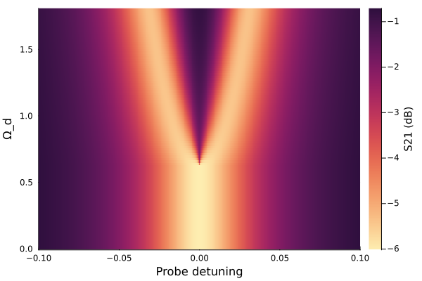

---

This page was generated using Literate.jl.