Cumulant approximations for the Kerr parametric oscillator

Let us compare the higher cumulant approximations for the Kerr parametric oscillator (KPO). The KPO is a model for a cavity with a Kerr nonlinearity and a parametric drive after one applied the Rotating Wave approximation. For this we use the QuantumCumulants and the QuantumCumulantsExt module in HarmonicBalance.

using QuantumCumulants, HarmonicBalance, Plots

first order cumulant

Let us define the Hamiltonian of the KPO using QuantumCumulants.

h = FockSpace(:cavity)
@qnumbers a::Destroy(h)
@variables Δ::Real U::Real G::Real κ::Real
param = [Δ, U, G, κ]

H_RWA = (-Δ + U) * a' * a + U * (a'^2 * a^2) / 2 - G * (a' * a' + a * a) / 2
ops = [a, a']

2-element Vector{QuantumCumulants.QSym}:
 a
 a′

We can now compute the mean-field equations for the KPO using the meanfield function from QuantumCumulants. We need the complete the system equations of moition using the complete function.

eqs_RWA = meanfield(ops, H_RWA, [a]; rates=[κ], order=1)
eqs_completed_RWA = complete(eqs_RWA)

∂ₜ(⟨a⟩) = (G*im)*⟨a′⟩ + ((-U + Δ)*im)*⟨a⟩ - 0.5⟨a⟩*κ + (-U*im)*⟨a′⟩*(⟨a⟩^2)
∂ₜ(⟨a′⟩) = ((U - Δ)*im)*⟨a′⟩ + (-G*im)*⟨a⟩ - 0.5⟨a′⟩*κ + (U*im)*(⟨a′⟩^2)*⟨a⟩

To compute the steady states of the KPO, we use HarmonicBalance. We define the HomotopyContinuation problem using the Problem.

fixed = (U => 0.001, κ => 0.002)
varied = (Δ => range(-0.03, 0.03, 100), G => range(1e-5, 0.02, 100))
problem_c1 = HarmonicBalance.Problem(eqs_completed_RWA, param, varied, fixed)

2 algebraic equations for steady states
Variables: aᵣ, aᵢ
Parameters: Δ, U, G, κ

This gives us the phase

result = get_steady_states(problem_c1, WarmUp())
plot_phase_diagram(result; class="stable")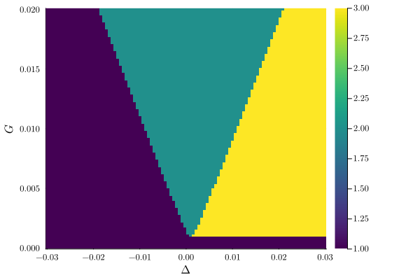

second order cumulant

The next order cumulant can be computed by setting the order keyword.

ops = [a]
eqs_RWA = meanfield(ops, H_RWA, [a]; rates=[κ], order=2)
eqs_c2 = complete(eqs_RWA)
problem_c2 = HarmonicBalance.Problem(eqs_c2, param, varied, fixed)

5 algebraic equations for steady states
Variables: aᵣ, aᵢ, a⁺aᵣ, aaᵣ, aaᵢ
Parameters: Δ, U, G, κ

Which gives us the phase diagram

result = get_steady_states(problem_c2, WarmUp())
plot_phase_diagram(result; class="stable", clim=(0, 4))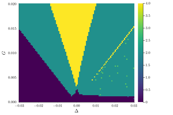

However, the phase diagram seems to wrong. Indeed, plotting, the photon number a⁺aᵣ shows that and additional state with the negative photon number is stable. However, the this is unphysical.

fixed = (U => 0.001, κ => 0.002, G => 0.01)
varied = (Δ => range(-0.03, 0.03, 200))
problem_c2 = HarmonicBalance.Problem(eqs_c2, param, varied, fixed)
result = get_steady_states(problem_c2, TotalDegree())
plot(result; y="a⁺aᵣ", class="stable")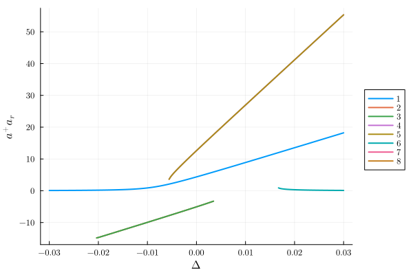

Let us classify the solutions having negative photon numbers. That way we can filter out these solutions.

classify_solutions!(result, "a⁺aᵣ < 0", "neg photon number");
plot(result; y="aᵣ", class="stable", not_class="neg photon number")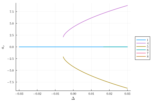

third order cumulant

Similarly, for third order

ops = [a]
eqs_RWA = meanfield(ops, H_RWA, [a]; rates=[κ], order=3)
eqs_c3 = complete(eqs_RWA)

fixed = (U => 0.001, κ => 0.002, G => 0.01)
varied = (Δ => range(-0.03, 0.03, 50))
problem_c3 = HarmonicBalance.Problem(eqs_c3, param, varied, fixed)
result = get_steady_states(problem_c3, TotalDegree())
classify_solutions!(result, "a⁺aᵣ < 0", "neg photon number");
plot(result; y="a⁺aᵣ", class="stable")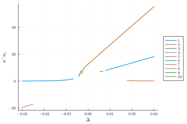

---

This page was generated using Literate.jl.